How to Use VLOOKUP in Google Sheets: A Step-by-Step Guide

VLOOKUP in Google Sheets lets you search for a value in the first column of a range and return a matching value from another column in the same row. It is one of the most useful functions in Google Sheets, and it can save a great deal of time and effort, especially with large datasets.

In this guide, we will walk through the basics of VLOOKUP in Google Sheets with examples to help you get started: the syntax, a basic lookup, using a cell reference, looking up data on another sheet, exact vs. approximate matches, common errors and fixes, and practical tips. It also includes a free VLOOKUP tester that shows exactly which row a formula lands on and why.

What Is VLOOKUP?

VLOOKUP stands for "vertical lookup." It searches down the first column of a range, often called the lookup column, until it finds the value you asked for, then moves across that row and returns the value from the column you choose.

This is particularly useful when you need to cross-reference data across different parts of your spreadsheet, such as pulling a price into an order form, an employee's department into a timesheet, or a customer's region into a sales report.

The Syntax of VLOOKUP

Before diving into examples, here is the syntax of the function, as documented in Google's VLOOKUP help page:

=VLOOKUP(search_key, range, index, [is_sorted])

The last argument is the one that trips people up. Google Sheets treats a missing is_sorted as TRUE, which means an approximate match. For most everyday lookups, such as finding a product, name, or ID, you want an exact match, so always type FALSE.

Example 1: Basic VLOOKUP in Google Sheets

Say you have a list of products and prices in a Google Sheet, and you want to find the price of a specific product.

Step 1: Set Up Your Data

Suppose your data is arranged like this, with products in column A and prices in column B.

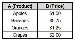
Step 2: Enter the VLOOKUP Formula

To find the price of Oranges, enter this formula in any empty cell:

=VLOOKUP("Oranges",A2:B5,2,FALSE)

Here, "Oranges" is the search_key. A2:B5 is the range containing the data. The 2 is the index for the Price column, because Price is the second column of the range. FALSE makes sure you get an exact match.

Result

The formula returns 1.25, the price of Oranges. If the cell is formatted as currency, it displays as $1.25.

Example 2: Using VLOOKUP With a Cell Reference

Instead of typing the search key into the formula, you can point to a cell that contains it. This makes the formula dynamic: change the cell, and the result updates.

Step 1: Set Up Your Data

Use the same product and price list as above.

Step 2: Reference the Search Key

Say you type Bananas in cell D1. Now write the formula like this:

=VLOOKUP(D1,A2:B5,2,FALSE)

D1 holds the search key, so the formula looks up whatever is in that cell.

Result

The formula returns 0.75, the price of Bananas. Type Grapes into D1 instead, and it returns 2. Pair this with a dropdown list in D1, made with Data validation, and you have a simple price checker.

Example 3: VLOOKUP With Multiple Sheets

VLOOKUP can also look up data on a different sheet within the same Google Sheets file.

Step 1: Set Up Your Data on a Different Sheet

Suppose you have a second sheet named Prices with the same product and price table in A1:B5.

Step 2: Enter the VLOOKUP Formula

To find the price of Grapes from that sheet, put the sheet name and an exclamation point in front of the range:

=VLOOKUP("Grapes",Prices!A2:B5,2,FALSE)

Prices!A2:B5 tells Google Sheets to use the range on the Prices sheet. If the sheet name contains spaces, wrap it in single quotes, as in 'Price List'!A2:B5.

Result

The formula returns 2, the price of Grapes, which displays as $2.00 when formatted as currency. To look up data in a completely separate spreadsheet file, combine VLOOKUP with IMPORTRANGE, which you will need to authorize the first time.

Exact Match vs. Approximate Match

With is_sorted set to FALSE, VLOOKUP returns the first row whose first column exactly matches the search key, ignoring upper and lower case. It also supports wildcards in exact-match mode: a question mark matches any single character, and an asterisk matches any sequence of characters, so "Gra*" finds Grapes.

With is_sorted set to TRUE, VLOOKUP assumes the first column is sorted in ascending order and returns the row with the largest value less than or equal to the search key. That is exactly what you want for tiered lookups, such as commission rates by sales amount or tax brackets by income. On unsorted data, however, it can quietly return the wrong row without any error, which is why FALSE is the safe default.

Common VLOOKUP Errors and How to Solve Them

Most VLOOKUP problems come down to a handful of causes.

The #N/A error occurs when VLOOKUP cannot find the search_key in the first column of the range. Double-check that your search_key and range match. To show a friendly message instead, wrap the formula: =IFERROR(VLOOKUP(D1,A2:B5,2,FALSE),"Not found").

The #REF! error happens when the index number is greater than the number of columns in the range. Make sure the index is within the range's column count.

Exact vs. approximate match is not an error message, but it is the most common source of wrong answers. If your data is not sorted, always use FALSE for is_sorted. Using TRUE, or leaving the argument out, can return incorrect results on unsorted data.

Free VLOOKUP Tester

Use the tester below to see how VLOOKUP behaves before you build it into your own sheet. It starts with the product list from this guide plus an in-stock column. Change the search key, the index, or is_sorted, and it highlights the row and cell VLOOKUP returns and explains the result. Try an index of 4 to see #REF!, a misspelled product to see #N/A, or "Gra*" to see a wildcard match.

Copy to Excel pastes the data and a live VLOOKUP formula that reads the search key, index, and is_sorted from cells, and it works the same way when pasted into Google Sheets. Print gives you a reference copy.

Tips for Using VLOOKUP Effectively

Keep your data organized. Make sure the first column of your range is where the search_key lives, and keep it free of duplicates, because VLOOKUP always returns the first match it finds.

Lock your range. Before copying a formula down a column, add dollar signs, as in $A$2:$B$5, so the range does not shift.

Use named ranges. If you use the same range in several VLOOKUP formulas, name it, for example PriceList, and write =VLOOKUP(D1,PriceList,2,FALSE).

Combine it with other functions. IFERROR handles missing values gracefully, and ARRAYFORMULA applies one VLOOKUP to a whole column at once, for example =ARRAYFORMULA(VLOOKUP(D2:D10,A2:B5,2,FALSE)).

Know when to use something else. VLOOKUP can only look to the right of the search column. When the value you need is to the left, or you want more flexible matching, use XLOOKUP, which Google Sheets also supports, or INDEX with MATCH.

Final Thoughts

VLOOKUP is an incredibly useful tool for quickly finding and retrieving data in Google Sheets. Whether you are managing inventory, analyzing data, or running a project, mastering VLOOKUP saves time and makes your workflow more efficient. With the steps and examples in this guide, you will be well on your way to becoming a VLOOKUP pro.

Ready to go further? Become an Excel expert here with free video courses that cover lookups, dashboards, and much more.

Sources

Google Docs Editors Help: VLOOKUP

Google Docs Editors Help: XLOOKUP function