Printable Excel Formulas Cheat Sheet

Use our Excel formula cheat sheet below to always have Excel solutions at your fingertips. If you use Excel for work, for business, or even just to organize your life, knowing the right formulas is the difference between spending 20 minutes on a task and spending 2. This cheat sheet covers every essential Excel formula category, with clear explanations and real examples you can use immediately.

Bookmark this page. You will come back to it.

Why Excel Formulas Matter

Excel has over 400 functions. You do not need to know all of them. You need to know the right ones, the ones that show up in real work, real businesses, and real decisions every single day. The formulas in this cheat sheet cover 95% of what most professionals will ever need. Master these and you will be faster, more accurate, and more valuable in any role.

Basic Arithmetic Formulas

These are the foundation. Everything else builds on them.

SUM

Adds up a range of numbers.

Formula: =SUM(A1:A10)

Example: You have monthly revenue figures in cells A1 through A12. =SUM(A1:A12) gives you your annual total in one second.

AVERAGE

Calculates the mean of a range of numbers.

Formula: =AVERAGE(A1:A10)

Example: You have daily sales figures for the month. =AVERAGE(A1:A30) tells you your average daily revenue without doing the math manually.

MIN and MAX

Returns the smallest or largest value in a range.

Formula: =MIN(A1:A10) and =MAX(A1:A10)

Example: You are reviewing a month of customer order values. =MIN tells you your smallest order. =MAX tells you your largest. Together they show you the spread of your data instantly.

COUNT and COUNTA

COUNT counts cells with numbers. COUNTA counts any non-empty cell.

Formula: =COUNT(A1:A10) and =COUNTA(A1:A10)

Example: You have a list of leads in column A. Some have phone numbers, some do not. =COUNTA tells you how many leads total. =COUNT tells you how many have a numeric value entered.

COUNTIF

Counts cells that meet a specific condition.

Formula: =COUNTIF(A1:A10, ">100")

Example: You have a column of order values. =COUNTIF(A1:A100, ">500") tells you exactly how many orders were over $500 without filtering or scrolling.

Text Formulas

Text functions are underrated. If you work with names, addresses, product codes, or any kind of text data, these save enormous amounts of time.

CONCATENATE and CONCAT

Joins multiple text strings into one.

Formula: =CONCATENATE(A1, " ", B1) or =CONCAT(A1, " ", B1)

Example: You have first names in column A and last names in column B. =CONCATENATE(A1, " ", B1) combines them into a full name in column C automatically across every row.

LEFT, RIGHT, and MID

Extracts characters from the left, right, or middle of a text string.

Formula: =LEFT(A1, 3) / =RIGHT(A1, 4) / =MID(A1, 2, 5)

Example: Your product codes in column A always start with a 3-letter category code. =LEFT(A1, 3) pulls just that code into a separate column so you can sort or filter by category.

LEN

Returns the number of characters in a text string.

Formula: =LEN(A1)

Example: You are cleaning a list of customer entries and need to flag any that are unusually short or long. =LEN quickly identifies cells that might have data entry errors.

TRIM

Removes extra spaces from text.

Formula: =TRIM(A1)

Example: You imported a contact list from another system and names have inconsistent spacing. =TRIM cleans every cell in one column without touching the content itself.

UPPER, LOWER, and PROPER

Converts text to uppercase, lowercase, or title case.

Formula: =UPPER(A1) / =LOWER(A1) / =PROPER(A1)

Example: Customer names came in as all caps from an old database. =PROPER(A1) converts "JOHN SMITH" to "John Smith" across thousands of rows instantly.

SUBSTITUTE

Replaces specific text within a string.

Formula: =SUBSTITUTE(A1, "old text", "new text")

Example: Your product names all include "2023" and you need to update them to "2024." =SUBSTITUTE handles every cell at once without find and replace.

Logical Formulas

Logical formulas make your spreadsheet think. They are where Excel goes from a calculator to a decision-making tool.

IF

Returns one value if a condition is true and another if it is false.

Formula: =IF(A1>100, "Yes", "No")

Example: You have a column of monthly sales figures. =IF(A1>10000, "Target Met", "Below Target") automatically flags every row based on performance. No manual review needed.

AND and OR

AND returns TRUE only if all conditions are true. OR returns TRUE if any condition is true.

Formula: =AND(A1>100, B1<50) / =OR(A1>100, B1<50)

Example: You want to flag customers who have placed more than 5 orders AND spent more than $1,000 total. =AND(B1>5, C1>1000) inside an IF formula gives you that filter automatically.

IFS

Tests multiple conditions in sequence without nesting multiple IF statements.

Formula: =IFS(A1>90, "A", A1>80, "B", A1>70, "C")

Example: You are building a performance rating system. =IFS lets you assign grades or tiers based on multiple thresholds cleanly, without the mess of stacking IF inside IF inside IF.

IFERROR

Returns a custom value if a formula produces an error.

Formula: =IFERROR(A1/B1, "N/A")

Example: You are dividing revenue by number of orders to get average order value. If orders is zero, Excel throws a division error. =IFERROR wraps the formula and shows "N/A" instead of an ugly error message.

Lookup Formulas

Lookup formulas are among the most powerful in Excel. They let you pull data from one place to another automatically, which is the core of almost every business spreadsheet.

VLOOKUP

Searches for a value in the first column of a range and returns a value from another column in the same row.

Formula: =VLOOKUP(A1, B1:D10, 3, FALSE)

Example: You have a product ID in column A and a price list on another sheet. =VLOOKUP pulls the correct price for each product ID automatically, no copy-pasting required.

HLOOKUP

Does the same as VLOOKUP but searches horizontally across rows instead of vertically down columns.

Formula: =HLOOKUP(A1, A1:J3, 2, FALSE)

Example: Your data is organized with months across the top row and categories down the side. =HLOOKUP finds the right month and returns the value from the row you specify.

INDEX and MATCH

A more powerful alternative to VLOOKUP. INDEX returns a value from a range at a specific row and column. MATCH finds the position of a value in a range. Together they are unstoppable.

Formula: =INDEX(C1:C10, MATCH(A1, B1:B10, 0))

Example: You need to look up a value to the left of your search column, which VLOOKUP cannot do. INDEX MATCH handles it without restructuring your data.

XLOOKUP

The modern replacement for VLOOKUP. Simpler syntax, more flexible, works in any direction.

Formula: =XLOOKUP(A1, B1:B10, C1:C10)

Example: You want to find a customer name and return their email address. =XLOOKUP finds the name in column B and returns the corresponding value from column C, left or right, no column number required.

FILTER

Returns all rows from a range that meet one or more conditions.

Formula: =FILTER(A1:C10, B1:B10>100)

Example: You have a full sales dataset and want to see only orders over $500 from a specific region. =FILTER returns exactly those rows dynamically. When your data updates, the filter updates automatically.

Date and Time Formulas

Date formulas are essential for tracking deadlines, calculating durations, and building reports that update automatically.

TODAY and NOW

Returns the current date or the current date and time.

Formula: =TODAY() and =NOW()

Example: You are building a project tracker. =TODAY() in a deadline column automatically calculates how many days are left until each deadline every time you open the file.

DATEDIF

Calculates the difference between two dates in days, months, or years.

Formula: =DATEDIF(A1, B1, "D")

Example: You want to know how long each customer has been with you. =DATEDIF(signup date, TODAY(), "M") gives you the number of months automatically for every customer in your list.

EDATE

Returns a date a specified number of months before or after a starting date.

Formula: =EDATE(A1, 3)

Example: You are tracking subscription renewals. Every contract starts on a different date and renews in 12 months. =EDATE(start date, 12) calculates every renewal date automatically.

EOMONTH

Returns the last day of the month a specified number of months from a date.

Formula: =EOMONTH(A1, 0)

Example: You need to set payment due dates at the end of the month of invoice. =EOMONTH(invoice date, 0) gives you the last day of that same month for every row.

NETWORKDAYS

Counts the number of working days between two dates, excluding weekends and optionally holidays.

Formula: =NETWORKDAYS(A1, B1)

Example: You want to know how many business days a project took from start to finish. =NETWORKDAYS gives you that number automatically without counting Saturdays and Sundays.

Financial Formulas

These formulas are built for business. Whether you are evaluating loans, investments, or cash flows, these save hours of manual calculation.

PMT

Calculates the regular payment amount for a loan.

Formula: =PMT(interest rate per period, number of periods, loan amount)

Example: You are considering a $50,000 equipment loan at 6% annual interest over 5 years. =PMT(6%/12, 60, -50000) tells you your exact monthly payment before you walk into the bank.

NPV

Calculates the net present value of a series of future cash flows.

Formula: =NPV(discount rate, value1, value2...)

Example: You are evaluating whether a new product line is worth launching. =NPV helps you determine whether the projected future profits, discounted to today's value, justify the upfront investment.

IRR

Returns the internal rate of return for a series of cash flows.

Formula: =IRR(values)

Example: You have projected cash flows for a new investment over five years. =IRR tells you the effective annual return of that investment so you can compare it against other options.

FV

Calculates the future value of an investment based on periodic payments and a fixed interest rate.

Formula: =FV(rate, periods, payment, present value)

Example: You are saving $1,000 per month at 5% annual interest. =FV tells you exactly what that savings will be worth in 10 years.

Statistical Formulas

Statistical formulas help you understand your data beyond the basics.

MEDIAN

Returns the middle value in a dataset.

Formula: =MEDIAN(A1:A10)

Example: You are looking at employee salaries. =AVERAGE can be skewed by one very high earner. =MEDIAN gives you the true middle value, which is often a more accurate picture of what most employees earn.

STDEV

Returns the standard deviation of a dataset, measuring how spread out the values are.

Formula: =STDEV(A1:A10)

Example: You are analyzing daily sales figures. A low standard deviation means your sales are consistent. A high one means they are volatile. Knowing which you have changes how you plan inventory and staffing.

PERCENTILE

Returns the value at a specific percentile in a dataset.

Formula: =PERCENTILE(A1:A10, 0.9)

Example: You want to know what order value puts a customer in the top 10% of your buyers. =PERCENTILE(order values, 0.9) gives you that threshold so you can identify and reward your best customers.

RANK

Returns the rank of a value within a list.

Formula: =RANK(A1, A1:A10, 0)

Example: You have monthly sales figures for your team. =RANK automatically assigns a position to each salesperson so you can build a leaderboard that updates itself every time numbers change.

Array Formulas

Array formulas perform calculations across multiple cells at once and are some of the most powerful tools in Excel.

SUMIF and SUMIFS

Adds values that meet one or more conditions.

Formula: =SUMIF(A1:A10, "North", B1:B10) / =SUMIFS(C1:C10, A1:A10, "North", B1:B10, ">100")

Example: You have sales data with regions in column A and revenue in column B. =SUMIF(A1:A100, "North", B1:B100) gives you total revenue from the North region only. =SUMIFS adds a second condition, like only orders over $500.

AVERAGEIF

Averages values that meet a condition.

Formula: =AVERAGEIF(A1:A10, ">100", B1:B10)

Example: You want to know the average order value for orders over $200 only. =AVERAGEIF isolates that segment without filtering or creating a separate table.

UNIQUE

Returns a list of unique values from a range, removing duplicates automatically.

Formula: =UNIQUE(A1:A10)

Example: You have a long list of customer names with many repeats. =UNIQUE returns each name once so you can see exactly how many distinct customers you have.

TRANSPOSE

Converts a vertical range to horizontal or vice versa.

Formula: =TRANSPOSE(A1:A10)

Example: Your data is organized in rows but your chart or report needs it in columns. =TRANSPOSE flips it instantly without copying and pasting manually.

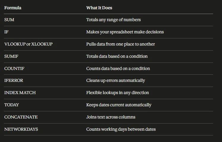
The Formulas That Matter Most for Business

If you only learn ten Excel formulas, make them these:

Frequently Asked Questions

What are the most important Excel formulas to learn first?

Start with SUM, AVERAGE, IF, and VLOOKUP. These four formulas cover the majority of everyday Excel tasks. Once you are comfortable with them, add SUMIF, COUNTIF, IFERROR, and INDEX MATCH to your toolkit and you will be able to handle almost any spreadsheet task you encounter.

What is the difference between VLOOKUP and INDEX MATCH?

VLOOKUP searches left to right only and requires you to specify a column number that can break if columns are inserted or deleted. INDEX MATCH is more flexible, can search in any direction, and does not break when your spreadsheet structure changes. For simple lookups VLOOKUP works fine. For anything complex, INDEX MATCH is the better habit.

What is the difference between VLOOKUP and XLOOKUP?

XLOOKUP is the modern replacement for VLOOKUP. It has simpler syntax, works in any direction, does not require a column number, and handles errors more cleanly. If you are using a recent version of Excel or Microsoft 365, learn XLOOKUP instead of VLOOKUP. Older versions of Excel do not support it.

Do Excel formulas work in Google Sheets?

Most do. SUM, AVERAGE, IF, VLOOKUP, INDEX MATCH, COUNTIF, SUMIF, and most text and date functions work identically in both. The main differences are that Google Sheets has some unique functions like QUERY and IMPORTRANGE that do not exist in Excel, while Excel has some advanced financial and statistical functions that Google Sheets does not fully support.

Why is my Excel formula showing an error?

The most common errors are: a reference to an empty or wrong cell, a division by zero, a VLOOKUP that cannot find the search value, or a mismatch between the data type the formula expects and what is actually in the cell. Wrap your formula in =IFERROR to handle errors gracefully, and double check that your cell references are pointing to the right place.

What is the fastest way to learn Excel formulas?

The fastest way is to learn by doing. Pick a real task you do at work, identify the formula that solves it, and build a spreadsheet around that one formula. Once it clicks in a real context, it sticks. Trying to memorize a formula list in isolation is the slowest approach. Apply each formula to something that actually matters to you and you will retain it immediately.

Can you combine multiple Excel formulas in one cell?

Yes, and this is where Excel becomes genuinely powerful. Nesting formulas inside each other, such as using IF inside SUMIF, or IFERROR around VLOOKUP, lets you build logic that handles complex real-world scenarios in a single cell. Start with simple formulas, get comfortable with each one individually, and then start combining them as your confidence grows.

What is IFERROR used for?

IFERROR wraps around any formula and returns a value you choose if that formula produces an error. Instead of seeing ugly error codes like #N/A or #DIV/0 in your spreadsheet, you see whatever you specify, such as "Not Found" or a blank cell. It is one of the most practical formulas in Excel for building clean, professional looking spreadsheets.

Take Your Excel Skills Further

Knowing formulas is the foundation. Knowing how to build real business tools in Excel, dashboards, trackers, financial models, and reporting systems, is what takes you from competent to genuinely valuable.

If you want to go deeper, our Excel course walks you through everything from the formulas in this guide to building complete business systems from scratch. You will learn how to think in Excel, not just how to copy formulas. Whether you are a small business owner who wants to get control of your numbers or a professional who wants to move faster and do more with data, the course gives you a practical, real-world education in Excel that you can apply from day one.

Every formula in this cheat sheet is covered in the course with hands-on exercises, real business examples, and step-by-step walkthroughs. No fluff, no filler, just the skills that actually matter.

Learn more about Excel here

How to make a project progress dashboard in Excel

All Excel formatting options explained

10 Tips for Creating Dashboards in Excel and Google Sheets

10 Excel Functions Every User Should Know